96.09%
Raw-audio Speech Commands
31.9k parameters. Six layers, width 32. No residual connections, gating, or normalization.
± 0.23 · 16,000 steps · full BPTTMemory takes time. A little look-ahead helps deep recurrent networks keep up.
1 Telepath2 New York University* shivang@telepath.com
The contributionA recurrent substrate. A better input path.
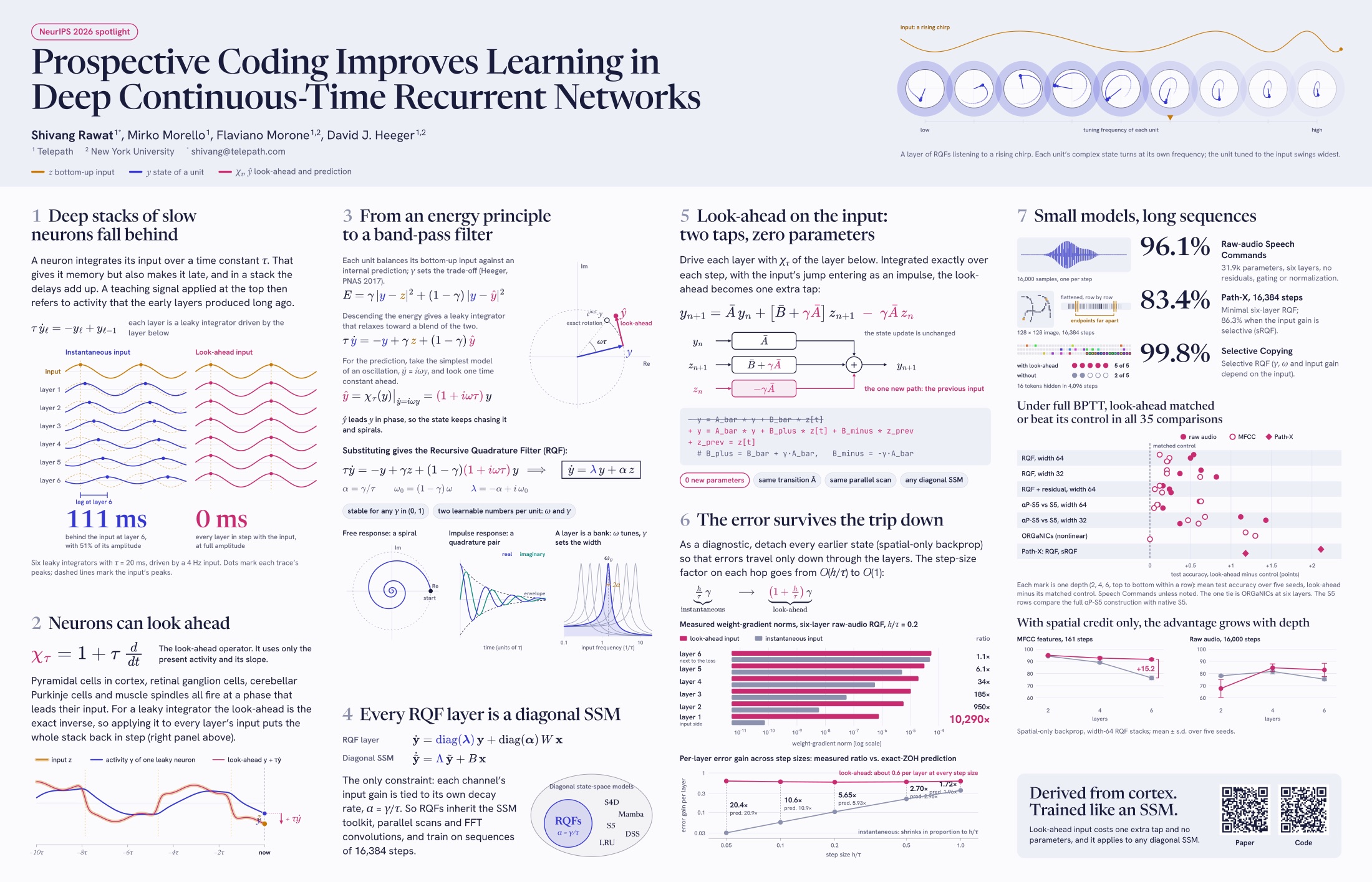
A neuron integrates its input over time. That gives it memory, but also makes it late. Stack these neurons, and the delays add up.
A teaching signal applied at the output refers to activity that early layers produced some time ago. The same temporal integration that makes a recurrent network useful can make a deep one harder to train.
Each layer is a leaky integratorτẏℓ = −yℓ + yℓ−1The layer below supplies the input.
lag at the final layer
of the input amplitude
Leaky integrators · τ = 20 ms
·
4 Hz input · ideal steady state
The prospective operator adds a signal’s local slope to its current value: z + τż. For a leaky integrator it is the exact differential inverse, cancelling its integration lag. As a time advance, it approximates z(t + τ) to first order.
It uses present activity and its slope. No future samples are needed. Prospective responses in cortex, retina, cerebellum, and muscle spindles motivate this construction.
An energy principle gives us a neuron. An oscillatory prediction gives it a rhythm.
A unit’s activity y balances a bottom-up input z and an internal prediction ŷ. The parameter γ sets their relative influence.
Descending this energy with respect to the state, holding the drives fixed, gives a leaky integrator that relaxes toward their blend:
Following the energy-based cortical theory of Heeger (PNAS, 2017); paper, Appendix A.1.
In the complex plane, ẏ = iωy rotates a state at a constant angular frequency. Its exact rotation over one time constant is eiωτy. The prospective operator gives its first-order version:
The prediction leads the state in phase. The state keeps chasing that prediction, producing a damped oscillation.
Look-ahead appears twice in this work: first in the recurrent prediction, then in the bottom-up input. Both input variants keep the same recurrent prediction.
Put the oscillatory prediction into the energy-derived dynamics. What remains is a stable, single-pole complex filter.
Two learnable dynamical parameters per unit: γ and ω. For real signals, the two components approximate a quadrature pair near resonance in the narrow-band regime.
Collect these filters into a layer and mix its inputs with W. You get a diagonal state-space model, with each channel’s input gain tied to its own decay rate.
Every RQF layer is a diagonal SSM. The inclusion is one-way: a general diagonal SSM need not have this pole–input-gain coupling.
Now use look-ahead a second time: drive each layer with z + τż. The recurrent dynamics stay the same. The input gets one extra path.
Exact impulse-ZOH update for an RQF channel.
= eλh,
= (α/λ)(
− 1). Initialize
the previous input to zero.
# coefficients from the same RQF parameters
B_plus  = B_bar + gamma * A_bar
B_minus = -gamma * A_bar

# two input taps, the same recurrent transition
y = A_bar * y + B_plus * z + B_minus * z_prev
z_prev = zThe added work is elementwise and linear in sequence length. For a general diagonal SSM, the extra coefficients are ±τB; the same construction applies beyond RQFs.
Hold each input constant over an integration interval of length h. At the boundary, the input changes from zn to zn+1, so its derivative is an impulse with that difference as its weight. Integrating the linear dynamics exactly propagates this impulse with . Since τα = γ, the extra contribution is γ(zn+1 − zn).
This is the paper’s impulse-ZOH convention, rather than a finite-difference approximation to a smooth derivative. See Section 3 and Appendix B for the derivation and the general diagonal-SSM form.
The smaller the time step, the less error an instantaneous input passes between layers.
To isolate this effect, detach earlier recurrent states and let errors travel only across layers within a step. Under this spatial-only backpropagation diagnostic, the input’s per-hop Euler coefficient changes from:
The exact ZOH update has the same leading-order scaling. Look-ahead removes this explicit step-size penalty at every spatial hop.
It removes a discretization-induced attenuation factor. Activation slopes, weights, and damping can still shrink the full gradient. Spatial-only training is a diagnostic; the main experiments also use full BPTT.
larger early-layer weight gradient
at layer 1 in this spatial-only diagnostic
The measured prospective per-hop error gain stays near 0.6 as the step size shrinks. The instantaneous gain falls roughly in proportion to h / τ, so their ratio grows. The ratio predicted from the exact ZOH coefficients follows this trend.
Spatial-only diagnostic, six-layer width-64 raw-audio RQF; paper, Table 10.
| h / τ | Prospective gain | Instantaneous gain | Measured ratio | Predicted ratio |
|---|---|---|---|---|
| 1.00 | 0.619 | 0.361 | 1.72× | 1.96× |
| 0.50 | 0.594 | 0.220 | 2.70× | 2.95× |
| 0.20 | 0.585 | 0.104 | 5.65× | 5.93× |
| 0.10 | 0.598 | 0.0565 | 10.59× | 10.91× |
| 0.05 | 0.624 | 0.0305 | 20.43× | 20.89× |
Per-hop gain is fitted over layers 6 to 2 from the RMS error norms. These are diagnostic measurements, not accuracy results.
From raw audio to nonlocal visual structure and content-aware memory. All numbers below come from the paper.
31.9k parameters. Six layers, width 32. No residual connections, gating, or normalization.
± 0.23 · 16,000 steps · full BPTTA minimal six-layer RQF reads a flattened 128 × 128 image. Input-selective sRQF reaches 86.31%.
± 1.71 · width 64 · full BPTTA four-layer selective RQF recalls 16 tokens hidden among 4,096 steps. Prospective input succeeds in 5/5 seeds; its control in 2/5.
± 0.07 · 33.0k parameters · full BPTTProspective variants match or improve mean test accuracy in all 35 comparisons on Speech Commands and Path-X.
RQF · αP-S5 · ORGaNICs · sRQFRQF · width 32 · Raw audio · 16,000 steps · Full BPTT
| Layers | Parameters | Prospective | Instantaneous | Difference |
|---|---|---|---|---|
| 2 | 23.5k | 94.59 ± 0.28% | 93.96 ± 0.28% | +0.63 pts |
| 4 | 27.7k | 95.66 ± 0.23% | 95.29 ± 0.22% | +0.37 pts |
| 6 | 31.9k | 96.09 ± 0.23% | 95.27 ± 0.22% | +0.82 pts |
Non-residual RQF stacks without normalization or gating. Source: paper, Table 6.
¹ Selective Copying accuracy is computed over seeds that exceed chance; success counts are reported separately. The αP-S5 comparison includes input-gain scaling, the second tap, and pole clipping. These are mean-accuracy comparisons, not claims of statistical significance.
An sRQF makes each channel’s input gain depend on the current input. For Path-X, that is the only selective component. For Selective Copying, the bandwidth γ and frequency ω also become input-dependent. The recurrence stays diagonal and retains its parallel scan; fixed-kernel FFT convolution applies to the time-invariant RQF.
Temporal integration gives continuous-time recurrent networks memory, but in deep stacks it also delays bottom-up signals and attenuates top-down errors. We compensate for this delay by making each layer’s bottom-up input prospective, and we develop Recursive Quadrature Filters (RQFs), biologically motivated temporal band-pass filters that are a special case of diagonal state-space models (SSMs). Starting from an energy model, we derive the RQF dynamics and show that each RQF is a band-pass filter whose learnable parameters control its tuning frequency and bandwidth. We then make each layer’s bottom-up input prospective using a parameter-free two-tap update that leaves the recurrent transition and parallel scan unchanged. We extend this correction to general diagonal SSMs and show that it mitigates depth-dependent gradient attenuation when temporal gradients are truncated, i.e., spatial-only backpropagation.
We evaluate the performance of RQFs, S5, and ORGaNICs (a nonlinear gated RNN with built-in attentional modulation and recurrent normalization) trained using full backpropagation through time (BPTT) and spatial-only backpropagation. Under full BPTT, the prospective variants of these models match or outperform their non-prospective controls in every configuration. A non-residual width-32 six-layer RQF achieves 96.09 ± 0.23% accuracy on raw-audio Speech Commands with 31.9k parameters; a width-64 six-layer RQF achieves 83.36 ± 1.71% on the 16,384-step Path-X task. We also introduce selective RQFs (sRQFs), which make each filter’s input gain and, optionally, its bandwidth and tuning frequency input-dependent while retaining the parallel scan. With the input gain alone, the same six-layer model achieves 86.31 ± 0.51% on Path-X; with all three input-dependent, a four-layer prospective sRQF solves Selective Copying (99.83 ± 0.07%). These results identify RQFs as a parameter-efficient recurrent substrate and prospective-input coding as an input-side correction for deep continuous-time recurrent networks.
@misc{rawat2026prospective,
  title = {Prospective Coding Improves Learning in Deep
           Continuous-Time Recurrent Networks},
  author = {Rawat, Shivang and Morello, Mirko and
            Morone, Flaviano and Heeger, David J.},
  year = {2026},
  eprint = {2609.04134},
  archivePrefix = {arXiv},
  primaryClass = {cs.LG},
  note = {NeurIPS 2026},
  url = {https://arxiv.org/abs/2609.04134}
}